Multiple myeloma example

POSE pipeline overview

(Single-modal) In this tutorial, we demonstrate how to perform the POSE pipeline on multiple myeloma (MM) RNA data restricted to the WEE1 neighborhood. This analysis entails the following:

1. Upload data

2. Compute pairwise sample (Euclidean) distances with respect to the WEE1 gene neigborhood.

3. Compute net pairwise sample (Euclidean) distance matrices

4. Convert net distances to a single sample pairwise similarity matrix

5. Compute scale-free DPT distance from similirities

6. Compue the POSE from the DPT distances

7. Probe the POSE

Aknowledgement

• The diffusion distance and pseudo-ordering is performed according to the lineage tracing algorithm presented in Haghverdi, et al. (2019).

• The code for computing the ordering is largely adopted from the scanpy implementation in Python.

Input

• X : RNA-Seq data matrix

• genelist : list of gene(s) of interest in X

• G : gene-gene (or protein-protein) interaction network

Algorithm

1. Upload input data

2. Compute sample-pairwise distances with respect to 1-hop-neighborhoods:

   • For each gene g in the genelist, compute $$d_{(g)}(i, j)$$ which is the distance of gene g’s 1-hop neighborhood (including self) between every two samples i and j.

3. Compute net sample-pairwise distances:

   • $$d(i,j) = |d_{(g)}(i, j)|$$ as the $L_1$ or $L_2$ norm of the vector of gene-1-hop-neighborhood distances for all genes g in the genelist.

4. Convert net sample-pairwise distances to standardized similarities:

   • $\sigma$ : Kernel width representing each data point’s accessible neighbors.

   • Set $\sigma$ normalization for each obs as the distance to its k-th neighbor : $$K_{ij}^{(d)} = \sqrt{\frac{2\sigma_i\sigma_j}{\sigma_i^2 + \sigma_j^2}}e^{-\frac{|d_{ij}^2|}{2(\sigma_i^2 + \sigma_j^2)}}$$ where for each observation $i$, $\sigma_i$ is the distance to its $k$-th nearest neighbor.

5. Compute scale-free DPT distance from similairites.

6. Compute POSE from DPT distances.

7. Probing the POSE entails:

   1. Perform BL-clustering on the final POSE

   2. Visualization (interactive)

First, import the necessary packages:

Load libraries

from pathlib import Path
import sys

import matplotlib.pyplot as plt
import networkx as nx
import numpy as np
import pandas as pd

from lifelines import KaplanMeierFitter
from lifelines.plotting import add_at_risk_counts
from lifelines.statistics import logrank_test, multivariate_logrank_test

If netflow has not been installed, add the path to the library:

sys.path.insert(0, Path(Path('.').absolute()).parents[3].resolve().as_posix())
# sys.path.insert(0, Path(Path('.').absolute()).parents[0].resolve().as_posix())

From the netflow package, we load the following modules:

• The InfoNet class is used to compute 1-hop neighborhood distances

• The Keeper class is used to store and manipulate data/results

import netflow as nf
import netflow.probe.clustering as nfc
import netflow.probe.visualization as nfv

A brief note on Keepers:

NetFlow’s data structure is called a Keeper. The Keeper, among other features, stores the feature data, sample-pairwise distances, sample-pairwise similarities, graphs, and miscellaneous data. The Keeper has sub-keepers specific to the type of data:

• DataKeeper

  • Stores features datasets where rows are features and columns are samples

  • All datasets in the global Keeper are expected to have the same samples

• DistanceKeeper

  • Stores sample-pairwise distances

  • All distances in the global Keeper are expected to have the same samples

• SimilarityKeeper

  • Stores sample-pairwise similarities

  • All similarities in the global Keeper are expected to have the same samples

• GraphKeeper

  • Stores graphs. Can be feature graphs or sample graphs - no checks or requirements are enforced.

• misc

  • A dictionary to store miscellaneous data or results that don’t directly fit into any of the previous sub-keepers

To load the data into the Keeper, you can first load the data into your workspace and then add it to the Keeper. I find it easier, and useful for repeating any analysis, to save the data so that it can be directly upload into the Keeper from the file. (Future versions of NetFlow will support more options for loading from file. Currently, the easiest is to save feature/distance/similarity data in a form that can be loaded by pandas, and to save graphs in the form of an edgelist with columns labelled 'source' and 'target'

Directories

MAIN_DIR = Path('.').resolve() / 'example_data' / 'MM' 
DATA_DIR = MAIN_DIR / 'data'

RNA_FNAME = DATA_DIR / 'rna_full.csv'
E_FNAME = DATA_DIR / 'edgelist_HPRD.csv'
CLIN_FNAME = DATA_DIR / 'clin_full.csv'

We first make a directory to save netflow results:

RESULTS_DIR = MAIN_DIR / 'netflow_results'

if not RESULTS_DIR.is_dir():
    RESULTS_DIR.mkdir()

NetFlow pipeline

Before starting the NetFlow pipeline, we initialize the keeper with the NetFlow results output directory:

keeper = nf.Keeper(outdir=RESULTS_DIR)

Step 1: Load data

Next, we load the data into the keeper:

Load the clinical data

Note: default NetFlow format for loading and storing feature data in the Keeper expects the data to be formatted with samples (a.k.a. observations) as columns and features as rows. However, the clinical data was saved with the transpose format (i.e., with features as columns and samples as rows). We specify this by setting the argument cols_as_obs=False.

keeper.load_data(CLIN_FNAME, label='clin', index_col=0, cols_as_obs=False)

The clinical data is now stored in the keeper’s DataKeeper and can be referenced with the key 'clin':

keeper.data['clin']

<netflow.keepers.keeper.DataView at 0x7f85c05164f0>

This returns the DataView. You can look into the code to see the different capabilities of the DataView class. In this tutorial I’ll demonstrate the main usage of the keeper and its subkeeper classes that you will likely be interested in:

The first usage is to extract a feature dataset from the keeper as a pandas DataFrame, with the .to_frame() method:

clin = keeper.data['clin'].to_frame()
clin.head()

	MMRF_1021_1_BM_CD138pos	MMRF_1029_1_BM_CD138pos	MMRF_1030_1_BM_CD138pos	MMRF_1031_1_BM_CD138pos	MMRF_1032_1_BM_CD138pos	MMRF_1033_1_BM_CD138pos	MMRF_1037_1_BM_CD138pos	MMRF_1048_1_BM_CD138pos	MMRF_1068_1_BM_CD138pos	MMRF_1073_1_BM_CD138pos	...	MMRF_2829_1_BM_CD138pos	MMRF_2830_1_BM_CD138pos	MMRF_2831_1_BM_CD138pos	MMRF_2832_1_BM_CD138pos	MMRF_2834_1_BM_CD138pos	MMRF_2836_1_BM_CD138pos	MMRF_2847_1_BM_CD138pos	MMRF_2848_1_BM_CD138pos	MMRF_2851_1_BM_CD138pos	MMRF_2853_1_BM_CD138pos
T	1.706849	2.726027	5.435616	3.641096	2.487671	0.59726	0.263014	4.849315	1.427397	7.380822	...	0.575342	0.391781	0.471233	0.156164	0.331507	0.383562	0.158904	0.413699	0.432877	0.156164
E	1	0	1	1	1	1	0	1	1	0	...	0	0	0	0	0	0	1	0	0	0
label	0	1	1	3	0	1	1	0	0	1	...	0	1	3	1	0	3	3	0	3	0
label_str	middle risk	lower risk	lower risk	higher risk	middle risk	lower risk	lower risk	middle risk	middle risk	lower risk	...	middle risk	lower risk	higher risk	lower risk	middle risk	higher risk	higher risk	middle risk	higher risk	middle risk

4 rows × 659 columns

Load the RNA data:

keeper.load_data(RNA_FNAME, label='RNA', index_col=0)

Similarly, the RNA data is also now stored in the keeper’s DataKeeper and can be referenced with the key 'RNA'

The RNA dataset can be extracted from the keeper in the same way as previously done for the clinical data, using the key 'RNA':

X = keeper.data['RNA'].to_frame()
X.head(2)

	MMRF_1021_1_BM_CD138pos	MMRF_1029_1_BM_CD138pos	MMRF_1030_1_BM_CD138pos	MMRF_1031_1_BM_CD138pos	MMRF_1032_1_BM_CD138pos	MMRF_1033_1_BM_CD138pos	MMRF_1037_1_BM_CD138pos	MMRF_1048_1_BM_CD138pos	MMRF_1068_1_BM_CD138pos	MMRF_1073_1_BM_CD138pos	...	MMRF_2829_1_BM_CD138pos	MMRF_2830_1_BM_CD138pos	MMRF_2831_1_BM_CD138pos	MMRF_2832_1_BM_CD138pos	MMRF_2834_1_BM_CD138pos	MMRF_2836_1_BM_CD138pos	MMRF_2847_1_BM_CD138pos	MMRF_2848_1_BM_CD138pos	MMRF_2851_1_BM_CD138pos	MMRF_2853_1_BM_CD138pos
A1CF	0.060523	0.071149	0.013625	0.018527	0.012452	0.034835	0.000000	0.010645	0.063212	0.036705	...	0.232524	0.033547	0.069779	0.025636	0.000000	0.059870	0.000000	0.000000	0.004791	0.004934
A2M	2.606094	3.318758	3.592433	0.256151	4.925435	2.071656	2.972069	0.235788	0.861647	0.614808	...	0.058550	0.066230	3.190138	0.301965	2.318094	0.887388	2.302761	0.674839	2.241157	0.023649

2 rows × 659 columns

As a side note, you can also extract a subset of the data - for a specified subset of features and/or samples:

keeper.data['RNA'].subset(observations=['MMRF_1029_1_BM_CD138pos', 'MMRF_1030_1_BM_CD138pos'], features=['WEE1', 'CDK1'])

	MMRF_1029_1_BM_CD138pos	MMRF_1030_1_BM_CD138pos
WEE1	1.398230	1.308308
CDK1	2.107045	1.587994

To see the labels of all feature datasets stored in the keeper:

keeper.data.keys()

dict_keys(['clin', 'RNA'])

Load the feature graph

Since the feature graph corresponds the RNA data, where each node in the graph corresponds to a gene in the RNA dataset, we use the label of the feature dataset for the graph as well, and set label='RNA':

keeper.load_graph(E_FNAME, label='RNA')

The graph can then be accessed from the keeper referenced by the key 'RNA':

print(keeper.graphs['RNA'])

Graph named 'RNA' with 8427 nodes and 33695 edges

Step 2: Compute sample-pairwise distances on the WEE1 neighborhood:

For any feature, we can compute distances, such as Wasserstein and Euclidean, between feature neighborhood profiles of every two observations.

Here’s a description of the arguments for computing distances over a neighborhood:

• data_key: the reference label of the feature dataset stored in the keeper that should be used to extract the feature profiles

• graph_key: the reference label of the feature graph stored in the keeper that should be used to determine the feature neighborhoods

• features : a list of features for which the neighborhood distances should be computed.

  • The distances are computed over the neighborhood of each feature in the list independently, and stored in keeper.misc.

  • Here, we only consider the WEE1 neighborhood, but alternative or additional genes could be added to this list.

• include_self: specify if the feature itself should be included in the neighborhood profile.

  • When computing transition probabilities, the weight of the feature itself ends up being excluded via the mass-action principle. When interested in the transition probabilities, set include_self = False. Otherwise, if interested in the distance between normalized profiles over the neighborhood, set include_self = True.

  • To take the mass-action approach when computing the Wasserstein distance, this should be set to False

For additional argument options, see the documentation.

data_key = 'RNA'
graph_key = 'RNA'
features = ['WEE1']

Now, we compute the Euclidean distance between feature neighborhoods:

The Euclidean metric is specified by the attribute metric. Any metric that can be passed to scipy.spatial.distance.cdist is acceptable. If no metric is specified, the default behavior is to use 'euclidean'.

keeper.euc_distance_pairwise_observation_feature_nbhd(data_key, graph_key, features=features, include_self=True, metric='euclidean')

netflow.methods.classes: 07/24/2025 10:57:38  AM | MSG |                                                           
classes:multiple_pairwise_observation_neighborhood_euc_distance:928 | >>> Loaded saved observation pairwise 1-hop  
neighborhood Euclidean distances from RNA_nbhd_euc_with_self profiles of size (216811, 1).                         

Note: If the keeper is instantiated with an output directory (outdir), the default behavior is to save the computed distances.

Any future computation with a keeper instantiated with the same output directory will first try to load these distances before recomputing. Be sure to change the output directory (outdir) if the samples or features change, or if you want to recompute the distances.

As a result, the sample-pairwise (Euclidean) distances with respect to 1-hop neighborhoods for each feature provided in features is stored in keeper.misc keyed by f"{data_key}_{label}_nbhd_euc_with{'' if include_self else 'out'}_self". The distances are stored in a stacked format as a pandas.DataFrame where column(s) are labeled by the features (in features) and the 2-multi-index indicate the labels of the observation between which the distance was computed.

We can see the Euclidean feature neighborhood distances have been added to keeper.misc:

keeper.misc.keys()

dict_keys(['RNA_nbhd_euc_with_self'])

And we can extract the computed distances as follows:

keeper.misc[f'{data_key}_nbhd_euc_with_self']

		WEE1
observation_a	observation_b
MMRF_1021_1_BM_CD138pos	MMRF_1029_1_BM_CD138pos	3.138194
	MMRF_1030_1_BM_CD138pos	3.758586
	MMRF_1031_1_BM_CD138pos	4.294601
	MMRF_1032_1_BM_CD138pos	2.474873
	MMRF_1033_1_BM_CD138pos	4.484517
...	...	...
MMRF_2847_1_BM_CD138pos	MMRF_2851_1_BM_CD138pos	4.353974
	MMRF_2853_1_BM_CD138pos	6.715387
MMRF_2848_1_BM_CD138pos	MMRF_2851_1_BM_CD138pos	3.539159
	MMRF_2853_1_BM_CD138pos	5.374954
MMRF_2851_1_BM_CD138pos	MMRF_2853_1_BM_CD138pos	6.097771

216811 rows × 1 columns

• Similarly, we can compute the Wasserstein distances between feature neighborhoods. To do so, uncomment below:

# keeper.wass_distance_pairwise_observation_feature_nbhd(data_key, graph_key, features=features, include_self=False)

Step 3: Extract net neighborhood distances

Distance from a single feature neighborhood

If we are interested in the distances with respect to a single feature neighborhood, as we are here (WEE1), we can extract the stacked-distance format from keeper.misc and add it to the distances in keeper.distances:

misc_key = f'{data_key}_nbhd_euc_with_self'

keeper.add_stacked_distance(keeper.misc[misc_key]['WEE1'], label=misc_key+'_WEE1')

We can now see this distance has been added to keeper.distances:

keeper.distances.keys()

dict_keys(['RNA_nbhd_euc_with_self_WEE1'])

Distance from norm of feature neighborhood distances

Alternatively, we can use the norm of the vector of neighborhood distances over multiple features as the final distance. (Note, this may also be performed for a single feature, and is equivalent to extracting the single neighborhood distances previously described.)

Uncomment below to perform

Summary of the arguments passed to compute the norm and save it as a distance:

• misc_key : Specify the key of the stacked RNA feature neighborhood Wasserstein distnaces stored in keeper.misc

• distance_label : Specify the key that the resulting distance is stored as in keeper.distances

• features : Option to select subset of features to include. If provided, restrict to norm over columns corresponding to features in the specified list. If None, use all columns. (In this demonstration, we use the default behavior and include all features that neighborhood distances were computed on.)

• method : Indicate which norm to compute, can be one of [‘L1’, ‘L2’, ‘inf’, ‘mean’, ‘median’]

First, we extract the norm of feature neighborhood distances, again demonstrated on the RNA-Euclidean distances:

# misc_key = f'{data_key}_nbhd_euc_with_self'
# distance_label = f"norm_{misc_key}"
# nf.methods.metrics.norm_features_as_sym_dist(keeper, misc_key, label=distance_label,
#                                              features=None, method='L1')

We can now see this distance has been added to keeper.distances:

# keeper.distances[distance_label].to_frame().head(2)

Feature profile distances

We can also compute sample-pairwise distances between feature profiles, using either the entire feature profile or restricted to a subset of the features.

For example, we use the Hallmark G2M Checkpoint pathway genes from msigdb (note WEE1 has been added at the end), which we reference as G2M_checkpoint_label = 'G2M'

G2M_checkpoint_label = 'G2M'

G2M_checkpoint_features = ['ABL1', 'AMD1', 'ARID4A', 'ATF5', 'ATRX', 'AURKA', 'AURKB', 'BARD1', 'BCL3', 
                           'BIRC5', 'BRCA2', 'BUB1', 'BUB3', 'CASP8AP2', 'CBX1', 'CCNA2', 'CCNB2', 'CCND1', 
                           'CCNF', 'CCNT1', 'CDC20', 'CDC25A', 'CDC25B', 'CDC27', 'CDC45', 'CDC6', 'CDC7', 
                           'CDK1', 'CDK4', 'CDKN1B', 'CDKN2C', 'CDKN3', 'CENPA', 'CENPE', 'CENPF', 'CHAF1A', 
                           'CHEK1', 'CHMP1A', 'CKS1B', 'CKS2', 'CTCF', 'CUL1', 'CUL3', 'CUL4A', 'CUL5', 'DBF4', 
                           'DDX39A', 'DKC1', 'DMD', 'DR1', 'DTYMK', 'E2F1', 'E2F2', 'E2F3', 'E2F4', 'EFNA5', 
                           'EGF', 'ESPL1', 'EWSR1', 'EXO1', 'EZH2', 'FANCC', 'FBXO5', 'FOXN3', 'G3BP1', 'GINS2', 
                           'GSPT1', 'H2AX', 'H2AZ1', 'H2AZ2', 'H2BC12', 'HIF1A', 'HIRA', 'HMGA1', 'HMGB3', 'HMGN2', 
                           'HMMR', 'HNRNPD', 'HNRNPU', 'HOXC10', 'HSPA8', 'HUS1', 'ILF3', 'INCENP', 'JPT1', 'KATNA1', 
                           'KIF11', 'KIF15', 'KIF20B', 'KIF22', 'KIF23', 'KIF2C', 'KIF4A', 'KIF5B', 'KMT5A', 'KNL1', 
                           'KPNA2', 'KPNB1', 'LBR', 'LIG3', 'LMNB1', 'MAD2L1', 'MAP3K20', 'MAPK14', 'MARCKS', 'MCM2', 
                           'MCM3', 'MCM5', 'MCM6', 'MEIS1', 'MEIS2', 'MKI67', 'MNAT1', 'MT2A', 'MTF2', 'MYBL2', 'MYC', 
                           'NASP', 'NCL', 'NDC80', 'NEK2', 'NOLC1', 'NOTCH2', 'NSD2', 'NUMA1', 'NUP50', 'NUP98', 
                           'NUSAP1', 'ODC1', 'ODF2', 'ORC5', 'ORC6', 'PAFAH1B1', 'PBK', 'PDS5B', 'PLK1', 'PLK4', 
                           'PML', 'POLA2', 'POLE', 'POLQ', 'PRC1', 'PRIM2', 'PRMT5', 'PRPF4B', 'PTTG1', 'PTTG3P', 
                           'PURA', 'RACGAP1', 'RAD21', 'RAD23B', 'RAD54L', 'RASAL2', 'RBL1', 'RBM14', 'RPA2', 'RPS6KA5', 
                           'SAP30', 'SFPQ', 'SLC12A2', 'SLC38A1', 'SLC7A1', 'SLC7A5', 'SMAD3', 'SMARCC1', 'SMC1A', 
                           'SMC2', 'SMC4', 'SNRPD1', 'SQLE', 'SRSF1', 'SRSF10', 'SRSF2', 'SS18', 'STAG1', 'STIL', 
                           'STMN1', 'SUV39H1', 'SYNCRIP', 'TACC3', 'TENT4A', 'TFDP1', 'TGFB1', 'TLE3', 'TMPO', 
                           'TNPO2', 'TOP1', 'TOP2A', 'TPX2', 'TRA2B', 'TRAIP', 'TROAP', 'TTK', 'UBE2C', 'UBE2S', 
                           'UCK2', 'UPF1', 'WRN', 'XPO1', 'YTHDC1', 'WEE1'] 

len(G2M_checkpoint_features)

201

If not all features are in the feature dataset, the subset of features that are present are used. To be sure of which features are used, we first restrict the list of features to those found in our dataset:

print(f"There are {len(set(G2M_checkpoint_features) & set(keeper.data['RNA'].feature_labels))} G2M checkpoint genes in the network")

There are 168 G2M checkpoint genes in the network

G2M_checkpoint_features = list(set(G2M_checkpoint_features) & set(keeper.data['RNA'].feature_labels))
len(G2M_checkpoint_features)

168

To compute the Euclidean distance between feature profiles, we use the following arguments:

• data_key: the reference label of the feature dataset stored in the keeper that should be used to extract the feature profiles

• features : a list of features for which the feature profile distances should be computed.

• label: reference label describing selected feature set added to the key used to reference the distance stored keeper.distances

Note: if computing the Wasserstein distance, graph_key must also be provided:

• graph_key: the reference label of the feature graph stored in the keeper that should be used to compute the Wasserstein distance between feature profiles.

Note: To compute Euclidean (or other supported distances) between all features in the dataset, use default values features=None and label=None.

See documentation on keeper.euc_distance_pairwise_observation_profile for more argument options and alternative supported metrics.

The Euclidean distance between the selected gene signature feature profiles are computed for the RNA feature data set as follows:

data_key = 'RNA'
features = G2M_checkpoint_features
label = G2M_checkpoint_label

keeper.euc_distance_pairwise_observation_profile(data_key, features=features, label=label)

Note: other distances are supported, see the documentation for keeper.euc_distance_pairwise_observation_feature_nbhd

We can see that the Euclidean distances were saved to the keeper, referenced by f'{data_key}_{label}_profile_euc':

keeper.distances.keys()

dict_keys(['RNA_nbhd_euc_with_self_WEE1', 'RNA_G2M_profile_euc'])

Similarly, uncomment to compute the Wasserstein distance between feature profiles:

# graph_key = 'RNA'
# data_key = 'RNA'
# features = G2M_checkpoint_features
# label = G2M_checkpoint_label

# keeper.wass_distance_pairwise_observation_profile(data_key, graph_key, features=features, label=label)

Step 4: Compute similarities from distances

Next, we convert the distance to a similarity. (to fuse multiple similarities, see the documentation)

Following the DPT approach, we use the individual sample-controlled normalization. We specify the number of nearest-neighbor samples to be considered in the computation by n_neighbors. See the documentation for a description of other arguments.

n_neighbors = 12

To compute the similarity for each of the computed distances, we iterate through the distances stored in keeper.distances:

for dd in keeper.distances:
    keeper.compute_similarity_from_distance(dd.label, n_neighbors, 'max',                                                    
                                            label=None, knn=False)

Now we can see that two similarities have been added to keeper.similarities:

keeper.similarities.keys()

dict_keys(['similarity_max12nn_RNA_nbhd_euc_with_self_WEE1', 'similarity_max12nn_RNA_G2M_profile_euc'])

Step 5: Compute diffusion distances

Next we show how to compute the scale-free DPT distance from a similarity. This entails computing the transition matrix associated with the similarity which is stored in the misc keeper, keyed by f"transitions_sym_{s.label}" (s refers to the similarity view (i.e., keeper.DistanceView), as used below).

To compute the diffusion distance for each similarity, we simply loop through the similarities stored in the keeper. See the documentation for a description of additional options.

for s in keeper.similarities:
    keeper.compute_dpt_from_similarity(s.label, density_normalize=True)

We can see that the multi-scale distances have been added to the keeper:

print(*keeper.distances.keys(), sep='\n')

RNA_nbhd_euc_with_self_WEE1
RNA_G2M_profile_euc
dpt_from_transitions_sym_similarity_max12nn_RNA_nbhd_euc_with_self_WEE1_density_normalized
dpt_from_transitions_sym_similarity_max12nn_RNA_G2M_profile_euc_density_normalized

Step 6: Compute the POSE

The POSER class is used to perform the iterative branching and keep track the branches and their splits. The final POSE, i.e., the Pseudo-Organizational StructurE of the observations is returned as a graph where each observation is represented as a node. The edges show the organizational relationship determined from the ordering (lineage tracing algorithm), called the backbone and nearest neighbors (alleviates strict assumptions of lineage tracing that do not apply and provides local affinity information).

Computing the pseudo-ordering backbone entails iteratively branching the data n_branches times, where n_branches is specified by the user.

See documentation for a description of other arguments. Here, I select my go-to settings.

We compute the POSE as follows:

mutual = True
k_mnn = 1
n_branches = 3

for key in keeper.distances.keys():
    if not key.startswith('dpt'):
        continue

    poser, G_poser_nn = keeper.construct_pose(key, n_branches=n_branches,
                                              min_branch_size=10,
                                              mutual=mutual, k_mnn=k_mnn,
                                              until_branched=True, verbose='ERROR', 
                                              root='density_inv', root_as_tip=True)

    g_name = f"POSE_{k_mnn}kmnn_{n_branches}branches_{key}"    
    print(g_name)
    G_poser_nn.name = g_name 
    # add the POSE graph to the keeper:
    keeper.add_graph(G_poser_nn, G_poser_nn.name)


    # for n_branches in [5, 9]:
    #     max_br_prev = max(list(dict(nx.get_node_attributes(G_poser_nn, 'branch')).values()))
    #     poser, G_poser_nn = keeper.construct_pose(key, n_branches=n_branches,
    #                                           min_branch_size=10,
    #                                           mutual=mutual, k_mnn=k_mnn,
    #                                           until_branched=True, verbose='ERROR', 
    #                                           root='density_inv', root_as_tip=True)
    #     max_br = max(list(dict(nx.get_node_attributes(G_poser_nn, 'branch')).values()))
    #     if max_br > max_br_prev:
    #         g_name = f"POSE_{k_mnn}kmnn_{n_branches}branches_{key}"
    #         print(g_name)
    #         G_poser_nn.name = g_name 
    #         # add the POSE graph to the keeper:
    #         keeper.add_graph(G_poser_nn, G_poser_nn.name)
    #         max_br_prev = max_br
    #     else:
    #         break

POSE_1kmnn_3branches_dpt_from_transitions_sym_similarity_max12nn_RNA_nbhd_euc_with_self_WEE1_density_normalized
POSE_1kmnn_3branches_dpt_from_transitions_sym_similarity_max12nn_RNA_G2M_profile_euc_density_normalized

We briefly go over some of the main arguments for consideration when computing the pose:

• root : You can specify which observation should be used as the root or the method to select the root. The default is to set the root as the central observation, determined as the observation with the smallest average distance to all other observations.

• min_branch_size : The minimum number of observations a branch must have to be considered for branching during the recursive branching procedure.

• split : If True, a branch is split according to its three tips. Otherwise, split the branch by determining a single branching off the main segment with respect to the tip farthest from the root.

• n_branches : The number of times to iteratively perform the branching, unless the process terminates earlier.

• until_branched : This is intended for compatibility with the scanpy implementation, where branching is iteratively attempted n_branches times. However, some iterations may not result in any further branching (e.g., if no split is found). We add the option (by setting until_branched = True) so that such iterations that do not result in further branching do not count toward the number of iterations performed. Thus, when until_branched = True, the iteration does not terminate until either a branch has been split or the process terminates.

See the documentation for a description of all possible arguments.

Note: here, we have computed the POSE with respect to the two scale-free DPT distances that were computed. In general, it can be computed with respect to any distance in the keeper.

Step 7: Probe the POSE

The topology of the POSE is return as G_poser_nn.

We highlight some of the node and edge attributes

Node attributes:

• 'branch' : Reference ID of the branch the observation belongs to.

• 'name' : Label of the observation the node corresponds to.

Edge attributes:

• 'connection’ : Takes one of the following values:

  • 'intra-branch' if the edge connects two observations in the same branch and

  • 'inter-branch' if the edge connects two observations in different branches.

• 'distance' :

• 'edge_origin' : Takes one of the following values:

  • 'POSE + NN'

  • 'POSE'

  • 'NN'

BL-clustering

We perform BL-clustering on each POSE (with Louvain resolution = 0.5) as follows:

for g in keeper.graphs:
    if not g.name.startswith('POSE'):
        continue
        
    # nfc.louvain_paritioned(g, 'branch', louvain_attr="louvain1", resolution=1.)
    nfc.louvain_paritioned(g, 'branch', louvain_attr="louvain0x5", resolution=0.5)
    nfc.louvain_paritioned(g, 'branch', louvain_attr="louvain0x1", resolution=0.1)

For example, we can see the attributes

• 'louvain0x5': Cluster index from the Louvain clustering with resolution = 0.5

• 'branch-louvain0x5': BL-cluster index (of the form i-j where i indicates the reference branch and j indicates the reference Louvain cluster

have been added to the POSE based on the WEE1-neighborhood as follows:

keeper.graphs['POSE_1kmnn_3branches_dpt_from_transitions_sym_similarity_max12nn_RNA_nbhd_euc_with_self_WEE1_density_normalized'].nodes[0]

{'branch': 4,
 'undecided': True,
 'name': 'MMRF_1021_1_BM_CD138pos',
 'unidentified': 1,
 'is_root': 'No',
 'pseudo-distance from root': 0.7780698011805295,
 'louvain0x5': 6,
 'branch-louvain0x5': '4-6',
 'louvain0x1': 3,
 'branch-louvain0x1': '4-3'}

Step 8: Visualizing the POSE

Interactive visualization

To start the interactive POSE visualization dashboard, we specify the key for the POSE graph as referenced in the keeper, and the key for the distance the POSE was computed off of, as stored in the keeper.

Note: You can switch to view other POSEs after the dashboard is initialized.

distance_key = 'dpt_from_transitions_sym_similarity_max12nn_RNA_nbhd_euc_with_self_WEE1_density_normalized'
# pose_key = f'POSE_1kmnn_5branches_{distance_key}'
pose_key = f'POSE_1kmnn_3branches_{distance_key}'

nf.render_pose(keeper, pose_key, distance_key, port=1786)

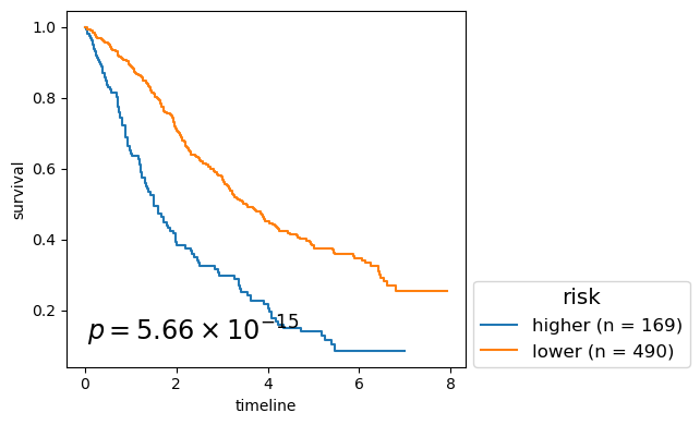
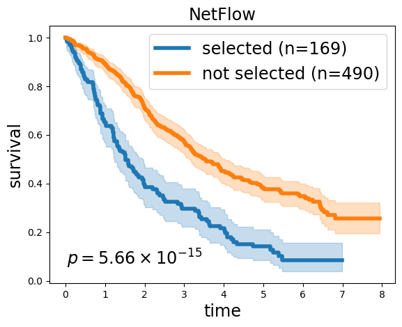
Kaplan-Meier Survival analysis from selected samples

Extract the survival time and event from the keeper:

clin = keeper.data['clin'].to_frame().T

selected = 'MMRF_2828_1_BM_CD138pos, MMRF_1580_1_BM_CD138pos, MMRF_1089_1_BM_CD138pos, MMRF_1927_1_BM_CD138pos, MMRF_1835_1_BM_CD138pos, MMRF_1499_1_BM_CD138pos, MMRF_1715_1_BM_CD138pos, MMRF_2667_1_BM_CD138pos, MMRF_2739_1_BM_CD138pos, MMRF_2394_1_BM_CD138pos, MMRF_2041_1_BM_CD138pos, MMRF_2681_1_BM_CD138pos, MMRF_1700_1_BM_CD138pos, MMRF_2535_1_BM_CD138pos, MMRF_1401_1_BM_CD138pos, MMRF_2818_1_BM_CD138pos, MMRF_2718_1_BM_CD138pos, MMRF_2476_1_BM_CD138pos, MMRF_1539_1_BM_CD138pos, MMRF_1831_1_BM_CD138pos, MMRF_2587_1_BM_CD138pos, MMRF_2200_1_BM_CD138pos, MMRF_1918_1_BM_CD138pos, MMRF_2532_1_BM_CD138pos, MMRF_2194_1_BM_CD138pos, MMRF_2015_1_BM_CD138pos, MMRF_1780_1_BM_CD138pos, MMRF_1641_1_BM_CD138pos, MMRF_2471_1_BM_CD138pos, MMRF_2621_1_BM_CD138pos, MMRF_1338_1_BM_CD138pos, MMRF_2754_1_BM_CD138pos, MMRF_2568_1_BM_CD138pos, MMRF_2225_1_BM_CD138pos, MMRF_1586_1_BM_CD138pos, MMRF_2639_1_BM_CD138pos, MMRF_1992_1_BM_CD138pos, MMRF_1683_1_BM_CD138pos, MMRF_2473_1_BM_CD138pos, MMRF_1541_1_BM_CD138pos, MMRF_1328_1_BM_CD138pos, MMRF_1617_1_BM_CD138pos, MMRF_2801_1_BM_CD138pos, MMRF_2776_1_BM_CD138pos, MMRF_1164_1_BM_CD138pos, MMRF_2452_1_BM_CD138pos, MMRF_2368_1_BM_CD138pos, MMRF_2813_1_BM_CD138pos, MMRF_1627_1_BM_CD138pos, MMRF_1851_1_BM_CD138pos, MMRF_1403_1_BM_CD138pos, MMRF_1677_1_BM_CD138pos, MMRF_1805_1_BM_CD138pos, MMRF_1359_1_BM_CD138pos, MMRF_2847_1_BM_CD138pos, MMRF_2076_1_BM_CD138pos, MMRF_1167_1_BM_CD138pos, MMRF_2272_1_BM_CD138pos, MMRF_1451_1_BM_CD138pos, MMRF_2401_1_BM_CD138pos, MMRF_2531_1_BM_CD138pos, MMRF_2692_1_BM_CD138pos, MMRF_1790_1_BM_CD138pos, MMRF_1819_1_BM_CD138pos, MMRF_2314_1_BM_CD138pos, MMRF_2245_1_BM_CD138pos, MMRF_2017_1_BM_CD138pos, MMRF_1710_1_BM_CD138pos, MMRF_1670_1_BM_CD138pos, MMRF_1727_1_BM_CD138pos, MMRF_2622_1_BM_CD138pos, MMRF_1664_1_BM_CD138pos, MMRF_2026_1_BM_CD138pos, MMRF_1797_1_BM_CD138pos, MMRF_2433_1_BM_CD138pos, MMRF_2746_1_BM_CD138pos, MMRF_2690_1_BM_CD138pos, MMRF_1389_1_BM_CD138pos, MMRF_1689_1_BM_CD138pos, MMRF_1269_1_BM_CD138pos, MMRF_1388_1_BM_CD138pos, MMRF_1822_1_BM_CD138pos, MMRF_1893_1_BM_CD138pos, MMRF_2676_1_BM_CD138pos, MMRF_1300_1_BM_CD138pos, MMRF_2807_1_BM_CD138pos, MMRF_1634_1_BM_CD138pos, MMRF_2436_1_BM_CD138pos, MMRF_1726_1_BM_CD138pos, MMRF_1461_1_BM_CD138pos, MMRF_1771_1_BM_CD138pos, MMRF_2691_1_BM_CD138pos, MMRF_1637_1_BM_CD138pos, MMRF_1971_1_BM_CD138pos, MMRF_2307_1_BM_CD138pos, MMRF_1645_1_BM_CD138pos, MMRF_2335_1_BM_CD138pos, MMRF_1842_1_BM_CD138pos, MMRF_1450_1_BM_CD138pos, MMRF_1534_1_BM_CD138pos, MMRF_1890_1_BM_CD138pos, MMRF_1932_1_BM_CD138pos, MMRF_2788_1_BM_CD138pos, MMRF_2778_1_BM_CD138pos, MMRF_2457_1_BM_CD138pos, MMRF_1424_1_BM_CD138pos, MMRF_2339_1_BM_CD138pos, MMRF_2836_1_BM_CD138pos, MMRF_2608_1_BM_CD138pos, MMRF_2605_1_BM_CD138pos, MMRF_2300_1_BM_CD138pos, MMRF_2251_1_BM_CD138pos, MMRF_2469_1_BM_CD138pos, MMRF_2698_1_BM_CD138pos, MMRF_1453_1_BM_CD138pos, MMRF_2817_1_BM_CD138pos, MMRF_1886_1_BM_CD138pos, MMRF_1644_1_BM_CD138pos, MMRF_1810_1_BM_CD138pos, MMRF_1251_1_BM_CD138pos, MMRF_1432_1_BM_CD138pos, MMRF_1618_1_BM_CD138pos, MMRF_2769_1_BM_CD138pos, MMRF_1833_1_BM_CD138pos, MMRF_1031_1_BM_CD138pos, MMRF_2799_1_BM_CD138pos, MMRF_1286_1_BM_CD138pos, MMRF_2722_1_BM_CD138pos, MMRF_2781_1_BM_CD138pos, MMRF_1169_1_BM_CD138pos, MMRF_2787_1_BM_CD138pos, MMRF_1906_1_BM_CD138pos, MMRF_2574_1_BM_CD138pos, MMRF_2062_1_BM_CD138pos, MMRF_2039_1_BM_CD138pos, MMRF_2290_1_BM_CD138pos, MMRF_2643_1_BM_CD138pos, MMRF_1817_1_BM_CD138pos, MMRF_1671_1_BM_CD138pos, MMRF_1862_1_BM_CD138pos, MMRF_2455_1_BM_CD138pos, MMRF_1595_1_BM_CD138pos, MMRF_1668_1_BM_CD138pos, MMRF_1721_1_BM_CD138pos, MMRF_1879_1_BM_CD138pos, MMRF_2490_1_BM_CD138pos, MMRF_2201_1_BM_CD138pos, MMRF_1082_1_BM_CD138pos, MMRF_2341_1_BM_CD138pos, MMRF_1579_1_BM_CD138pos, MMRF_1364_1_BM_CD138pos, MMRF_1540_1_BM_CD138pos, MMRF_1837_1_BM_CD138pos, MMRF_2458_1_BM_CD138pos, MMRF_1736_1_BM_CD138pos, MMRF_1327_1_BM_CD138pos, MMRF_1682_1_BM_CD138pos, MMRF_2373_1_BM_CD138pos, MMRF_2174_1_BM_CD138pos, MMRF_2119_1_BM_CD138pos, MMRF_2706_1_BM_CD138pos, MMRF_2438_1_BM_CD138pos, MMRF_1755_1_BM_CD138pos, MMRF_2125_1_BM_CD138pos, MMRF_2595_1_BM_CD138pos, MMRF_1596_1_BM_CD138pos, MMRF_1079_1_BM_CD138pos, MMRF_2195_1_BM_CD138pos, MMRF_2211_1_BM_CD138pos'
selected = selected.split(', ')
print(len(selected))

other_samples = list(set(clin.index) - set(selected))

fig, ax = plt.subplots(1, 1) # , dpi=300)
kmf1 = KaplanMeierFitter()
kmf2 = KaplanMeierFitter()
kmf1.fit(clin.loc[selected, 'T'], event_observed=clin.loc[selected, 'E'], label=f'selected (n={len(selected)})')
kmf2.fit(clin.loc[other_samples, 'T'], event_observed=clin.loc[other_samples, 'E'], label=f'not selected (n={len(other_samples)})')

lr = logrank_test(clin.loc[selected, 'T'], clin.loc[other_samples, 'T'], 
                  event_observed_A=clin.loc[selected, 'E'], event_observed_B=clin.loc[other_samples, 'E'])

kmf1.plot(ax=ax, lw=4)
kmf2.plot(ax=ax, lw=4)

ax.set_title('NetFlow', fontsize='xx-large');
ax.set_xlabel('time', fontsize='xx-large');
ax.set_ylabel('survival', fontsize='xx-large');
# ax.legend(loc='lower left', fontsize='xx-large');
ax.legend(loc='upper right', fontsize='xx-large');

lrp = f"{lr.p_value:2.2e}"
if 'e' in lrp:
    lrp = r"$p = {0} \times 10^{{{1}}}$".format(*lrp.split('e'))
else:
    lrp = r"$p = {0}$".format(lrp)
# ax.text(0.05, 0.3, lrp, # f"p = {lr.p_value:2.2e}", 
ax.text(0.05, 0.05, lrp, # f"p = {lr.p_value:2.2e}", 
        transform=ax.transAxes, ha='left', va='bottom', fontsize='xx-large');# 


# fig.savefig(f'/Users/renae12/Downloads/mm_kmf.png', 
#             dpi=300, bbox_inches='tight', transparent=True)

169

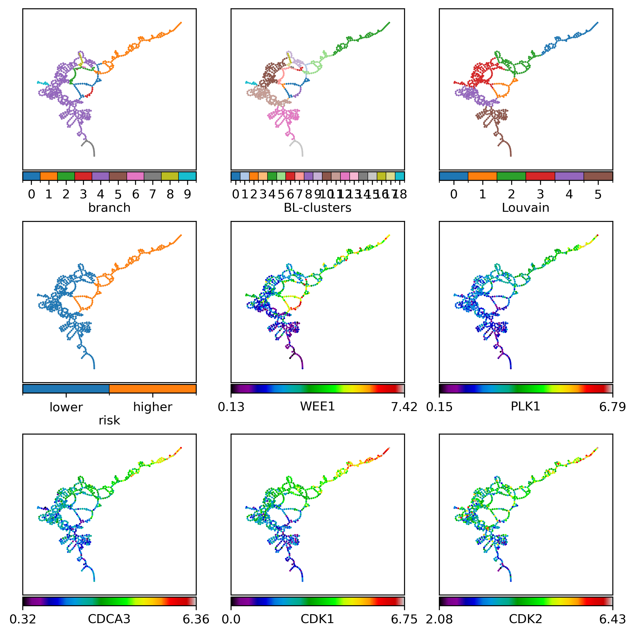
Panel visualization

pose_key = 'POSE_1kmnn_3branches_dpt_from_transitions_sym_similarity_max12nn_RNA_nbhd_euc_with_self_WEE1_density_normalized'
gg = keeper.graphs[pose_key]

selected = 'MMRF_2828_1_BM_CD138pos, MMRF_1580_1_BM_CD138pos, MMRF_1089_1_BM_CD138pos, MMRF_1927_1_BM_CD138pos, MMRF_1835_1_BM_CD138pos, MMRF_1499_1_BM_CD138pos, MMRF_1715_1_BM_CD138pos, MMRF_2667_1_BM_CD138pos, MMRF_2739_1_BM_CD138pos, MMRF_2394_1_BM_CD138pos, MMRF_2041_1_BM_CD138pos, MMRF_2681_1_BM_CD138pos, MMRF_1700_1_BM_CD138pos, MMRF_2535_1_BM_CD138pos, MMRF_1401_1_BM_CD138pos, MMRF_2818_1_BM_CD138pos, MMRF_2718_1_BM_CD138pos, MMRF_2476_1_BM_CD138pos, MMRF_1539_1_BM_CD138pos, MMRF_1831_1_BM_CD138pos, MMRF_2587_1_BM_CD138pos, MMRF_2200_1_BM_CD138pos, MMRF_1918_1_BM_CD138pos, MMRF_2532_1_BM_CD138pos, MMRF_2194_1_BM_CD138pos, MMRF_2015_1_BM_CD138pos, MMRF_1780_1_BM_CD138pos, MMRF_1641_1_BM_CD138pos, MMRF_2471_1_BM_CD138pos, MMRF_2621_1_BM_CD138pos, MMRF_1338_1_BM_CD138pos, MMRF_2754_1_BM_CD138pos, MMRF_2568_1_BM_CD138pos, MMRF_2225_1_BM_CD138pos, MMRF_1586_1_BM_CD138pos, MMRF_2639_1_BM_CD138pos, MMRF_1992_1_BM_CD138pos, MMRF_1683_1_BM_CD138pos, MMRF_2473_1_BM_CD138pos, MMRF_1541_1_BM_CD138pos, MMRF_1328_1_BM_CD138pos, MMRF_1617_1_BM_CD138pos, MMRF_2801_1_BM_CD138pos, MMRF_2776_1_BM_CD138pos, MMRF_1164_1_BM_CD138pos, MMRF_2452_1_BM_CD138pos, MMRF_2368_1_BM_CD138pos, MMRF_2813_1_BM_CD138pos, MMRF_1627_1_BM_CD138pos, MMRF_1851_1_BM_CD138pos, MMRF_1403_1_BM_CD138pos, MMRF_1677_1_BM_CD138pos, MMRF_1805_1_BM_CD138pos, MMRF_1359_1_BM_CD138pos, MMRF_2847_1_BM_CD138pos, MMRF_2076_1_BM_CD138pos, MMRF_1167_1_BM_CD138pos, MMRF_2272_1_BM_CD138pos, MMRF_1451_1_BM_CD138pos, MMRF_2401_1_BM_CD138pos, MMRF_2531_1_BM_CD138pos, MMRF_2692_1_BM_CD138pos, MMRF_1790_1_BM_CD138pos, MMRF_1819_1_BM_CD138pos, MMRF_2314_1_BM_CD138pos, MMRF_2245_1_BM_CD138pos, MMRF_2017_1_BM_CD138pos, MMRF_1710_1_BM_CD138pos, MMRF_1670_1_BM_CD138pos, MMRF_1727_1_BM_CD138pos, MMRF_2622_1_BM_CD138pos, MMRF_1664_1_BM_CD138pos, MMRF_2026_1_BM_CD138pos, MMRF_1797_1_BM_CD138pos, MMRF_2433_1_BM_CD138pos, MMRF_2746_1_BM_CD138pos, MMRF_2690_1_BM_CD138pos, MMRF_1389_1_BM_CD138pos, MMRF_1689_1_BM_CD138pos, MMRF_1269_1_BM_CD138pos, MMRF_1388_1_BM_CD138pos, MMRF_1822_1_BM_CD138pos, MMRF_1893_1_BM_CD138pos, MMRF_2676_1_BM_CD138pos, MMRF_1300_1_BM_CD138pos, MMRF_2807_1_BM_CD138pos, MMRF_1634_1_BM_CD138pos, MMRF_2436_1_BM_CD138pos, MMRF_1726_1_BM_CD138pos, MMRF_1461_1_BM_CD138pos, MMRF_1771_1_BM_CD138pos, MMRF_2691_1_BM_CD138pos, MMRF_1637_1_BM_CD138pos, MMRF_1971_1_BM_CD138pos, MMRF_2307_1_BM_CD138pos, MMRF_1645_1_BM_CD138pos, MMRF_2335_1_BM_CD138pos, MMRF_1842_1_BM_CD138pos, MMRF_1450_1_BM_CD138pos, MMRF_1534_1_BM_CD138pos, MMRF_1890_1_BM_CD138pos, MMRF_1932_1_BM_CD138pos, MMRF_2788_1_BM_CD138pos, MMRF_2778_1_BM_CD138pos, MMRF_2457_1_BM_CD138pos, MMRF_1424_1_BM_CD138pos, MMRF_2339_1_BM_CD138pos, MMRF_2836_1_BM_CD138pos, MMRF_2608_1_BM_CD138pos, MMRF_2605_1_BM_CD138pos, MMRF_2300_1_BM_CD138pos, MMRF_2251_1_BM_CD138pos, MMRF_2469_1_BM_CD138pos, MMRF_2698_1_BM_CD138pos, MMRF_1453_1_BM_CD138pos, MMRF_2817_1_BM_CD138pos, MMRF_1886_1_BM_CD138pos, MMRF_1644_1_BM_CD138pos, MMRF_1810_1_BM_CD138pos, MMRF_1251_1_BM_CD138pos, MMRF_1432_1_BM_CD138pos, MMRF_1618_1_BM_CD138pos, MMRF_2769_1_BM_CD138pos, MMRF_1833_1_BM_CD138pos, MMRF_1031_1_BM_CD138pos, MMRF_2799_1_BM_CD138pos, MMRF_1286_1_BM_CD138pos, MMRF_2722_1_BM_CD138pos, MMRF_2781_1_BM_CD138pos, MMRF_1169_1_BM_CD138pos, MMRF_2787_1_BM_CD138pos, MMRF_1906_1_BM_CD138pos, MMRF_2574_1_BM_CD138pos, MMRF_2062_1_BM_CD138pos, MMRF_2039_1_BM_CD138pos, MMRF_2290_1_BM_CD138pos, MMRF_2643_1_BM_CD138pos, MMRF_1817_1_BM_CD138pos, MMRF_1671_1_BM_CD138pos, MMRF_1862_1_BM_CD138pos, MMRF_2455_1_BM_CD138pos, MMRF_1595_1_BM_CD138pos, MMRF_1668_1_BM_CD138pos, MMRF_1721_1_BM_CD138pos, MMRF_1879_1_BM_CD138pos, MMRF_2490_1_BM_CD138pos, MMRF_2201_1_BM_CD138pos, MMRF_1082_1_BM_CD138pos, MMRF_2341_1_BM_CD138pos, MMRF_1579_1_BM_CD138pos, MMRF_1364_1_BM_CD138pos, MMRF_1540_1_BM_CD138pos, MMRF_1837_1_BM_CD138pos, MMRF_2458_1_BM_CD138pos, MMRF_1736_1_BM_CD138pos, MMRF_1327_1_BM_CD138pos, MMRF_1682_1_BM_CD138pos, MMRF_2373_1_BM_CD138pos, MMRF_2174_1_BM_CD138pos, MMRF_2119_1_BM_CD138pos, MMRF_2706_1_BM_CD138pos, MMRF_2438_1_BM_CD138pos, MMRF_1755_1_BM_CD138pos, MMRF_2125_1_BM_CD138pos, MMRF_2595_1_BM_CD138pos, MMRF_1596_1_BM_CD138pos, MMRF_1079_1_BM_CD138pos, MMRF_2195_1_BM_CD138pos, MMRF_2211_1_BM_CD138pos'
selected = selected.split(', ')

record = pd.DataFrame({k: dict(gg.nodes.data(k)) for k in ['name', 'branch', 'branch-louvain0x1', 'louvain0x1']}).set_index('name')
record = record.rename(columns={'louvain0x1': 'Louvain', 'branch-louvain0x1': 'BL-clusters'})

record['BL-clusters'] = record['BL-clusters'].map(dict(zip(sorted(record['BL-clusters'].unique()), range(record['BL-clusters'].nunique()))))
record['risk'] = ['higher' if k in set(selected) else 'lower' for k in record.index]
# record


# clin_g[['NF_selected']].to_csv(NETFLOW_RESULTS_DIR / 'netflow_selected_samples_POSE_1kmnn_5branches_dpt_from_transitions_sym_similarity_max5nn_WEE1_RNA_nbhd_euc_with_self_density_normalize.csv', header=True, index=True)

s = selected
s = None

nodelist = list(gg)
pos = nx.layout.kamada_kawai_layout(gg)


if s is None:
    border_linewidths = 0
else:
    s_names = {gg.nodes[k]['name']: k for k in gg}
    s = set([s_names[k] for k in s])
    border_linewidths = [0.24 if k in s else 0. for k in nodelist]  # : scalar or sequence (default=1.0) 
bordercolors = 'k' # ['k' if k in s else cc for k, cc in zip(nl, nc)] # [None | scalar | sequence] (default = node_color)                    


fts = pd.concat([record.replace({'risk': {'higher': 1, 'lower': 0}}), 
                 keeper.data['RNA'].subset(features=['WEE1',  'PLK1', 'CDCA3', 'CDK1', 'CDK2', 
                                          # 'ATAD2', 'SPAG5', 'RAD21', 'MCM4', 
                                          # 'GABARAPL1', 'RALGDS', 'SNUPN', 'CHIC2', 'FARSA',
                                         ]).T], axis=1)
fts = fts.rename(index={gg.nodes[k]['name']: k for k in gg})
fts = fts.loc[nodelist]

# fig, axes = plt.subplots(1, 6, figsize=(13, 2.5), layout='constrained', dpi=300)
fig, axes = plt.subplots(3, 3, figsize=(7, 7), layout='constrained', dpi=300)


for (ft_label, ft), ax in zip(fts.iteritems(), np.ravel(axes)):
    if ft_label in ['Louvain', 'BL-clusters', 'branch']:
        node_cmap = 'tab10' if ft.nunique() <= 10 else 'tab20' if ft.nunique() <= 20 else 'nipy_spectral'
        ntm= None
    elif ft_label == 'risk':
        node_cmap = 'tab10' 
        ntm = {0: 'lower', 1: 'higher'}
    else:
        node_cmap = 'nipy_spectral'
        ntm = None
    nfv.plot_topology(gg, pos=pos, ax=ax, nodelist=nodelist, node_size=2.2, # 4.3, # 2.3, 
                      node_color=ft.values, edge_color='lightgray', node_cbar=True, 
                      node_cbar_kws={'location': 'bottom', 'orientation': 'horizontal', 'pad': 0.01},
                      node_cbar_label=ft_label, 
                      node_cmap=node_cmap,
                      node_ticklabels_mapper=ntm,
                      border_linewidths=border_linewidths, bordercolors=bordercolors,
                     )

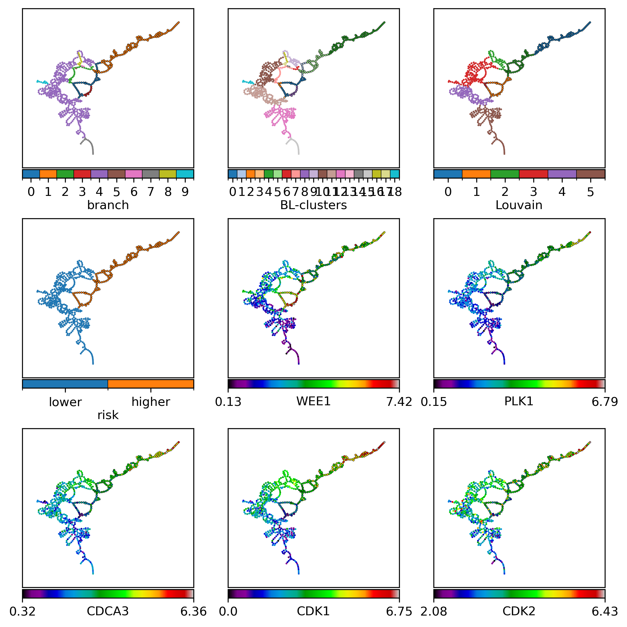
Visualization annotating selected samples:

s = selected
# s = None

nodelist = list(gg)
pos = nx.layout.kamada_kawai_layout(gg)


if s is None:
    border_linewidths = 0
else:
    s_names = {gg.nodes[k]['name']: k for k in gg}
    s = set([s_names[k] for k in s])
    border_linewidths = [0.24 if k in s else 0. for k in nodelist]  # : scalar or sequence (default=1.0) 
bordercolors = 'k' # ['k' if k in s else cc for k, cc in zip(nl, nc)] # [None | scalar | sequence] (default = node_color)                    


fts = pd.concat([record.replace({'risk': {'higher': 1, 'lower': 0}}), 
                 keeper.data['RNA'].subset(features=['WEE1',  'PLK1', 'CDCA3', 'CDK1', 'CDK2', 
                                          # 'ATAD2', 'SPAG5', 'RAD21', 'MCM4', 
                                          # 'GABARAPL1', 'RALGDS', 'SNUPN', 'CHIC2', 'FARSA',
                                         ]).T], axis=1)
fts = fts.rename(index={gg.nodes[k]['name']: k for k in gg})
fts = fts.loc[nodelist]

# fig, axes = plt.subplots(1, 6, figsize=(13, 2.5), layout='constrained', dpi=300)
fig, axes = plt.subplots(3, 3, figsize=(7, 7), layout='constrained', dpi=300)


for (ft_label, ft), ax in zip(fts.iteritems(), np.ravel(axes)):
    if ft_label in ['Louvain', 'BL-clusters', 'branch']:
        node_cmap = 'tab10' if ft.nunique() <= 10 else 'tab20' if ft.nunique() <= 20 else 'nipy_spectral'
        ntm= None
    elif ft_label == 'risk':
        node_cmap = 'tab10' 
        ntm = {0: 'lower', 1: 'higher'}
    else:
        node_cmap = 'nipy_spectral'
        ntm = None
    nfv.plot_topology(gg, pos=pos, ax=ax, nodelist=nodelist, node_size=2.2, # 4.3, # 2.3, 
                      node_color=ft.values, edge_color='lightgray', node_cbar=True, 
                      node_cbar_kws={'location': 'bottom', 'orientation': 'horizontal', 'pad': 0.01},
                      node_cbar_label=ft_label, 
                      node_cmap=node_cmap,
                      node_ticklabels_mapper=ntm,
                      border_linewidths=border_linewidths, bordercolors=bordercolors,
                     )

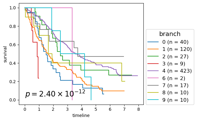
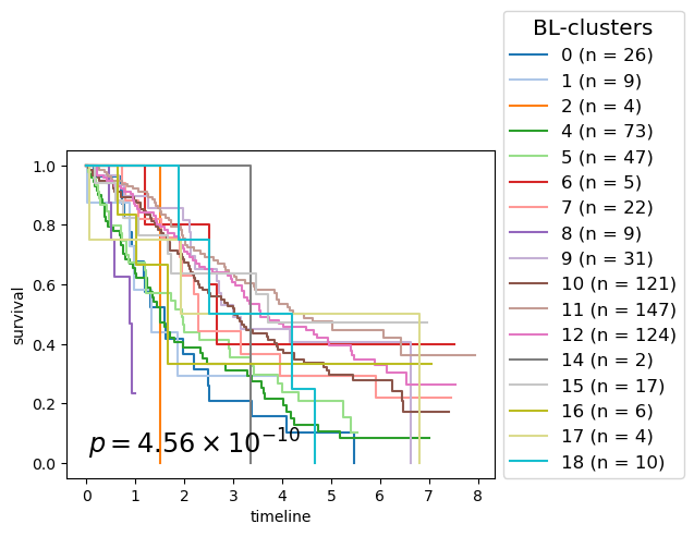
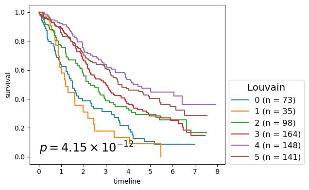
clin_g = pd.concat([clin[['T', 'E']], record], axis=1)

for cl in record.columns:
    if clin_g[cl].nunique() <= 10:
        cmap = plt.cm.tab10
    elif clin_g[cl].nunique() <= 20:
        cmap = plt.cm.tab20
    else:
        cmap = None # plt.cm.Pastel2
        
    colors = dict(zip(sorted(clin_g[cl].unique()), cmap.colors))
    
    p_mv = multivariate_logrank_test(clin_g['T'], clin_g[cl], event_observed=clin_g['E'])
    
    nfv.KM_between_groups(clin_g['T'], clin_g['E'], clin_g[cl], 
                          min_group_size=2, 
                          figsize=(6, 4), show_censors=False, ci_show=False, 
                          show_at_risk_counts=False, precision=17, 
                          ttl=None, # f"{cl} (multivariate p = {p_mv.p_value:.3E})", 
                          xlabel=None, colors=colors, ax=None,
                         )
    
    lrp = f"{p_mv.p_value:2.2e}"
    if 'e' in lrp:
        lrp = r"$p = {0} \times 10^{{{1}}}$".format(*lrp.split('e'))
    else:
        lrp = r"$p = {0}$".format(lrp)
    # ax.text(0.05, 0.3, lrp, # f"p = {lr.p_value:2.2e}", 
    plt.gca().text(0.05, 0.05, lrp, # f"p = {lr.p_value:2.2e}", 
            transform=plt.gca().transAxes, ha='left', va='bottom', fontsize='xx-large');# 
    plt.gca().legend(fontsize='large', title=cl, title_fontsize='x-large',
                     loc=(1.02, 0.), # loc='upper right', 
                    )
    
# multivariate p : 
# . branch - 2.398E-12    
# . BL-clusters - 4.561E-10
# . Louvain - 4.155E-12
# . risk - 5.659E-15